


Using Python in Excel to Run Monte Carlo Stock Return Simulations

Python in Excel is a new feature where one can write Python code in Excel to process data and perform other tasks. The Python written in Excel appears to be running in a Jupyter Notebook - and the experience is really similar.
Getting Started with Python in Excel
Python in Excel is currently not a released feature. More information can be found in the Excel Blog Announcement.
To use Python in Excel, join the Microsoft 365 Insider Program. Choose the Beta Channel Insider level to get the latest builds of the Excel application.
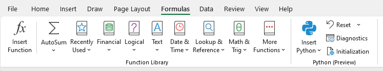
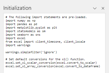
Python Menu and Initialization
The Python options can be found on the Formula menu.
The Initialization button will show what libraries are loaded. Pandas, Seaborn, matplotlib, etc. are initialized by default.
Creating Python in Excel
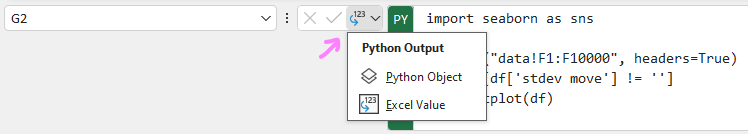
Select any empty cell and type =PY( to trigger Python mode. The output of the cell will be the value of the last Python statement. There is a button next to a Python cell that selects what kind of output the cell will produce. Python Objects can be used in other Python cells, and Excel Values will be visible to the user in the case of images and can be used by other Excel functions.
Creating a Monte Carlo Simulation
Retrieve Stock Data
Analyze Daily Returns
Monte Carlo Sampling From Distribution
Let's start up Excel and get started!
Retrieve Stock Data
Rename the sheet from Sheet1 to dashboard.
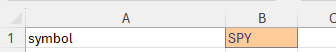
Create a symbol field to be used as input. SPY is used as an example on this project.
Create another sheet to be used as the data source sheet.
Rename the sheet from Sheet2 to data.
Setting Up data
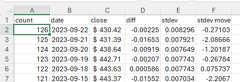
count
Count down from 126 to 1 in the first column. Top row is 126 and the next row is set to =A2-1. Copy this value down the sheet.
date and close
Set cell B2 to
=SORT(STOCKHISTORY(dashboard!B1, TODAY() - 10000, TODAY(), 0, 0, 0, 1), 1, -1)
This retrieves the stock price data for the symbol specified in the dashboard sheet and sorts the dates in reverse order.
diff
Calculate the percent daily returns. Using the percent daily returns is essential as we need to be able to compare the returns of a stock when the price is different values (i.e. 100 to 101 should be the same as 200 to 202).
=IF(ISNUMBER(C3), (C2-C3)/C3, "")
Copy the formula down 10000 rows!
stdev
Calculate the standard deviation of the last 20 days of percent daily returns. This gives us the 20 day historical volatility for the stock price for each day.
=IF(ISNUMBER(D22), STDEV.S(D3:D22), "")
Copy the formula down 10000 rows!
stdev_move
Calculate the move for the day in comparison to the standard deviation of the last 20 days. This will be used for creating a distribution that we can sample for the Monte Carlo simulation.
=IF(ISNUMBER(E2), D2/E2, "")
Again, copy the formula down 10000 rows!
Data Analysis on the dashboard Sheet
Switch back to the dashboard sheet.
Most data about returns and volatility is expressed as an annualized number to allow us to compare one instrument to another no matter what time frame is being examined.
Let's get the most recent standard deviation and put it into B2.
=data!E2
To calculate the annualized volatility, we multiply our standard deviation with the square root of the number of time periods in a year. The average trading year has 252 days in it, so we multiply by square root of 252 in B3.
=B2*SQRT(252)
If we were working with weekly data, we would multiply by the square root of 52. If we had minute data, we multiply by the square root of the number of days (252) multiplied by the number of minutes in a trading day (6.5 hours * 60 minutes), or SQRT(252*6.5*60).
The last closing price is in cell B4 for reference.
=data!C2
The total count of data points is in cell B6.
=COUNT(data!F:F)
Understanding the Distribution of Returns
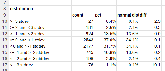
Stock returns do not follow a log normal distribution - they have really "fat tails." Sigma is the Greek letter used representing one standard deviation and looks like this: σ. We can show that the standard deviation of returns is not normal.
Column A contains labels:
>= 3 stdev
>= 2 and < 3 stdev
>= 1 and < 2 stdev
>= 0 and < 1 stdev
< 0 and > -1 stddev
<= -1 and > -2 stddev
<= -2 and > -3 stddev
<= -3 stddev
Column B counts the standard deviation moves in the data sheet.
=COUNTIF(data!F:F, ">=3")
=COUNTIFS(data!F:F, ">=2", data!F:F, "<3")
=COUNTIFS(data!F:F, ">=1", data!F:F, "<2")
=COUNTIFS(data!F:F, ">0", data!F:F, "<1")
=COUNTIFS(data!F:F, "<=0", data!F:F, ">-1")
=COUNTIFS(data!F:F, "<=-1", data!F:F, ">-2")
=COUNTIFS(data!F:F, "<=-2", data!F:F, ">-3")
=COUNTIF(data!F:F, "<=-3")
Column C is the percentage of occurrences of the range of standard deviations. It uses the count of the data from cell B6 performed in the initial analysis.
Copy and paste the following in rows C10-C17
=B10/$B$6
We can find this diagram by looking up the normal distribution on Wikipedia. We can see the letter sigma (σ) in there describing the distribution.
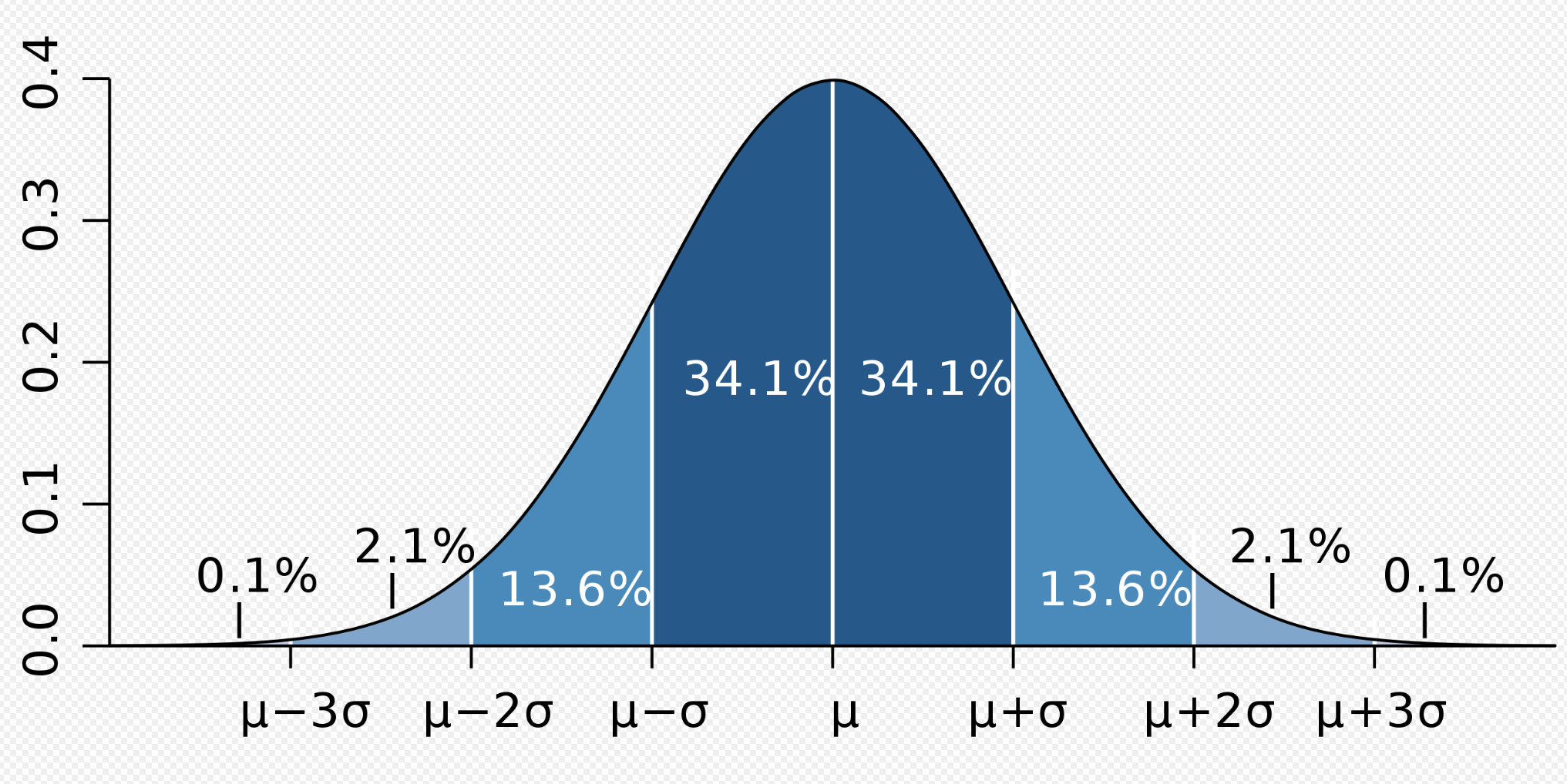
(“Probability measure,” 2023)
Enter the percentages into column D
We now can compare the percentage we saw in the returns versus the percentage of returns that should be in the range if the returns were normal.
Copy and paste the following in rows E10-E17
=ABS(C10-D10)/D10
A +3 sigma move shows up about three times more often in the SPY return data than a normal distribution. A -3 sigma move shows up 10 times more often!
Almost all financial mathematical models are based on normal or log normal distributions, as these are easy to work with and well understood, but it is not reality. We have shown that the distributions in SPY are not normal and have really fat tails.
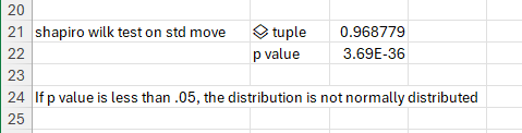
There is also a test called Shapiro-Wilk that determines if a set of data is normally distributed, and it is really easy to implement with Python in Excel.
In cell B21 type =PY(. This will trigger the cell to go into Python mode. Then make the cell look like the following...
from scipy.stats import shapiro

df = xl("data!F1:F10000", headers=True)
df = df[df['stdev_move'] != '']

shapiro(df['stdev_move'])
Remember to finish editing by pressing Ctrl+Enter.
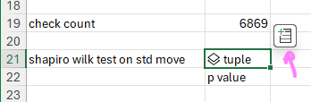
Since we left the return type as a Python object, we need to add an Excel value by selecting the cell, clicking on the table button that pops up, and selecting arrayPreview.
The first value is the test statistic and the second value is the p-value. Since the p-value is less than .05, the distribution is not normally distributed.
Charting Excel Data Using Python
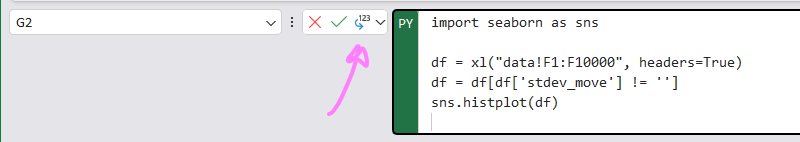
Seaborn library makes it pretty easy to plot a histogram. In cell G2.
import seaborn as sns

df = xl("data!F1:F10000", headers=True)
df = df[df['stdev_move'] != '']
sns.histplot(df)
The xl function is a special Python in Excel that will capture the data in the referenced cells. It seems to be pretty good at bringing in the data in the correct type. Ranges are imported as Pandas DataFrames and singular values have the correct type.
Ensure you select the Excel value from the output dropdown!
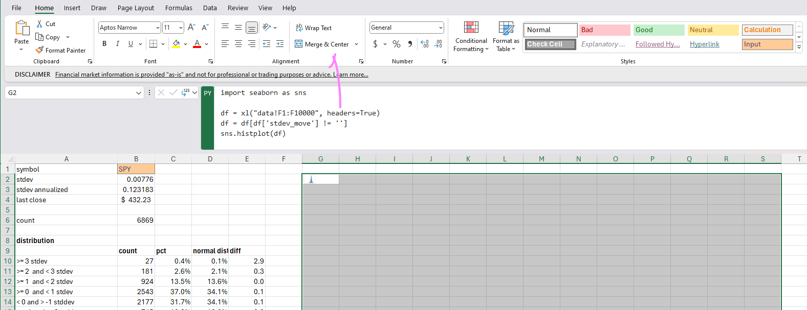
Excel will generate a little tiny histogram that needs to be expanded so you can see it. Select a number of cells of the desired chart size and then click the Merge and Center button.
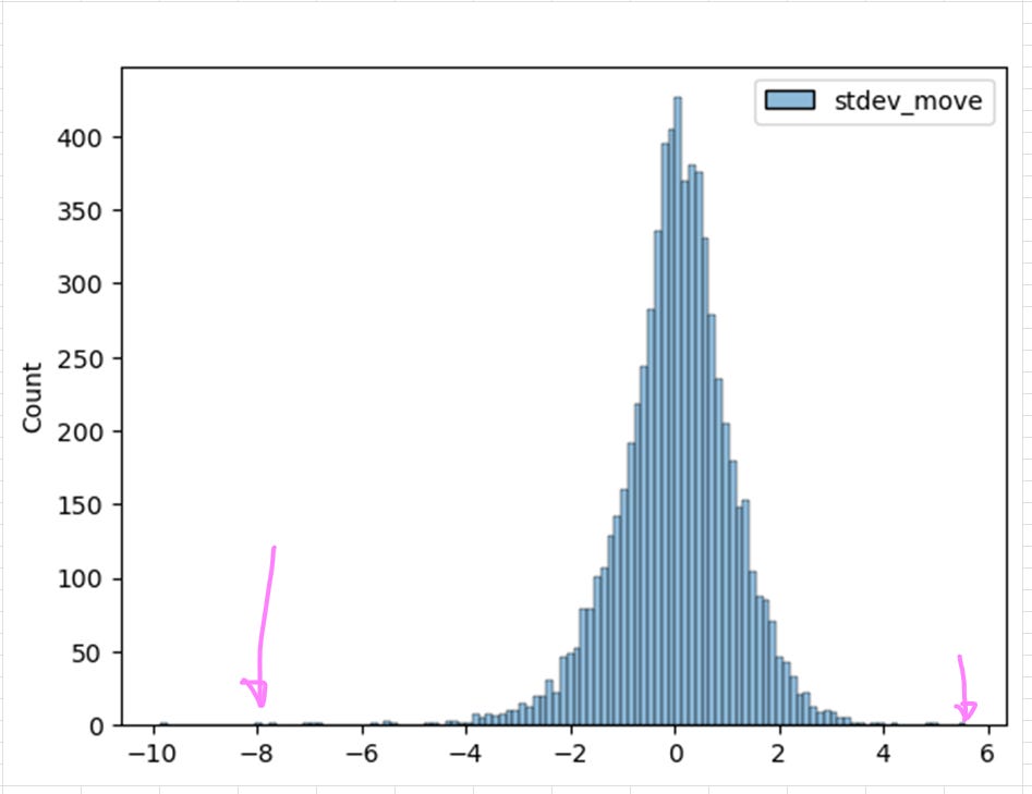
Now we can visibly see the fat tails of the distribution!
It is nice to have a little chart for you to see the current movement of the instrument. In cell G41 enter to produce a daily price chart of the last 126 days.
import seaborn as sns

df = xl("data!A1:F10000", headers=True)
df = df[df['count'] != '']
sns.regplot(df[['count', 'close']], x='count', y='close')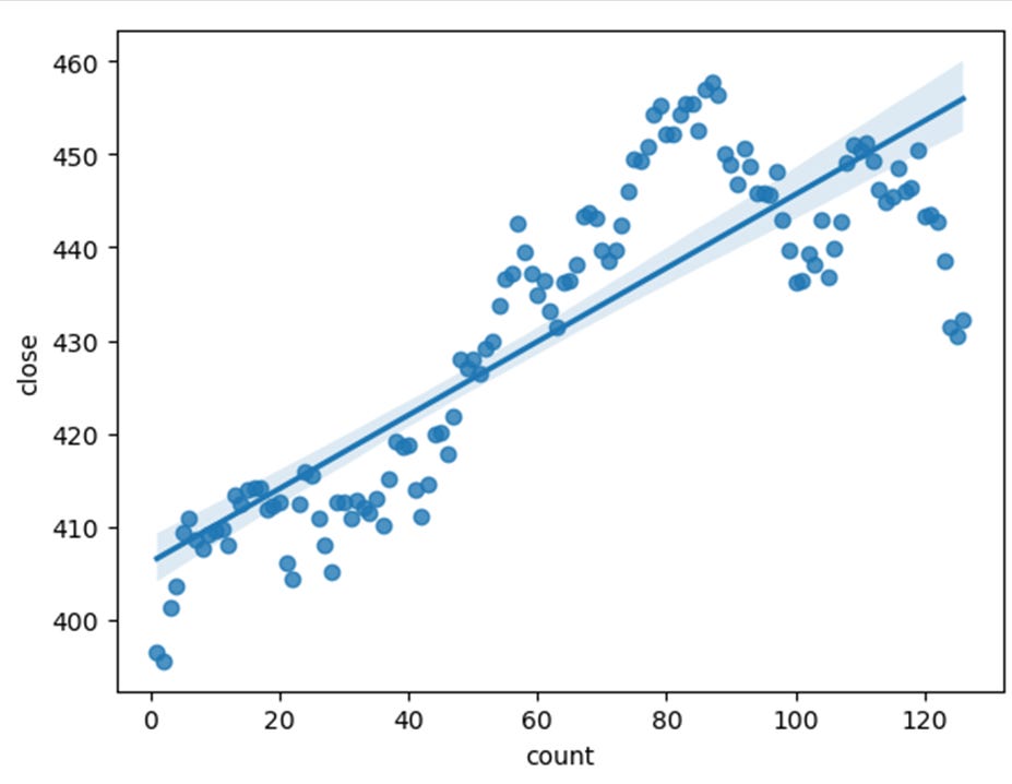
We can see that SPY has been moving up over the last two quarters.
Monte Carlo Simulation Using Python
Create input values for the Monte Carlo simulation.
n_simulations
n_time_steps
price_level
n_simulations - number of simulations to run
n_time_steps - number of time steps (in our case it is days) to simulate
price_level - price level to predict the probability of the price being above or below
Enter the following in cell G80
df = xl("data!F1:F10000", headers=True)
df = df[df['stdev_move'] != '']

# get the input from the cells
n_simulations = xl("B80")
n_time_steps = xl("B81")
price_level = xl("B82")

# get the current standard deviation
current_stdev = xl("B2")

# create the first column, time step 0, using the last closing price
last_close = [xl("B4")] * n_simulations
df_mc = pd.DataFrame(last_close, columns=[f't{0:02d}'])

for time_step in range(n_time_steps):
    col_name = f't{time_step+1:02d}'
    col_name_before = f't{time_step:02d}'

    # sample the returns from our observed distribution
    df_mc.insert(len(df_mc.columns), col_name, list(df['stdev_move'].sample(n_simulations, replace=True, ignore_index=True)), True)

    # create a new time step by adding the sampled return times the previous time step to the previous time step
    df_mc[col_name] = df_mc[col_name_before] + (df_mc[col_name_before] * current_stdev * df_mc[col_name])

# create a table of the probability of the time step being above or below our price level
probabilities = []
for c in df_mc.columns:
    p = len(df_mc[df_mc[c] >= price_level]) / n_simulations
    probabilities.append([c, p, 1 - p])

pd.DataFrame(probabilities, columns=['time_step', 'p_above', 'p_below'])
Make sure you select Excel Value as the output.
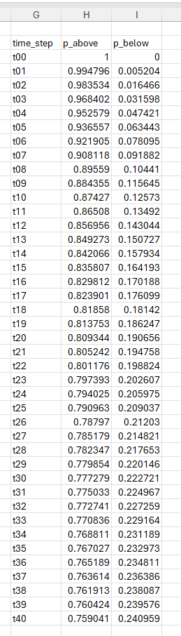
And here are our results! SPY is currently trading at 432.23. There is a 12.5% chance that it will be under 420 in 10 days. There is a whopping 24% chance that in 40 days, the price will be under 420.
It is important to remember that this probability is the terminal value of the price. Price could have gone below 420 and then back above in a simulation, but we are only checking the price on a particular time step. Determining the probability of a price being breached at any time will be left as an exercise for the reader.
References
Probability measure. (2023, March 15). In Wikipedia. https://en.wikipedia.org/wiki/Probability_measure#